The Shockingly Simple Math Behind Your Sales Pipeline

Most business leaders think about their sales pipeline the way they think about the weather: something to observe, worry about, and hope goes well. They check it in their CRM, feel good when it’s big and nervous when it’s thin, and make decisions largely on instinct.
But your pipeline is not the weather. It is a system. And like any system, it follows predictable mathematical laws. Once you understand the math, you stop guessing and start engineering your revenue.
The law in question has been around since 1961. It was discovered by an MIT operations researcher named John Little, and it describes how things flow through any queuing system: factory floors, hospital waiting rooms, airport security lines. It turns out it describes your sales pipeline just as well.
Want to crunch your numbers? Check out our calculator.
Sales Pipeline Calculator
Little’s Law, Explained
Little’s Law states:
L = λ × W
Where:
- L is the average number of items in the system
- λ (lambda) is the average rate at which items arrive
- W is the average time each item spends in the system
In plain English: the size of any queue is just the arrival rate multiplied by the time spent waiting.
For your sales pipeline, this translates directly:
Pipeline Size = Lead Flow Rate × Average Sales Cycle Length
That’s it. If you add 10 new deals per month to your pipeline, and your average deal takes 3 months to close (or die), you will always have roughly 30 deals in your pipeline at any given time. Little’s Law says so.
One important word in that sentence is “average.” Little’s Law works on averages, not on any individual deal. In practice, some deals close in three weeks and others drag on for six months. Some months you get eight inbound leads and some months you get two. The law describes the expected behavior of the system over time, not a guarantee about any given week or quarter. We will come back to this.
Adding the Close Rate
Little’s Law tells you pipeline size. But what you actually care about is closed revenue. To get there, you need one more variable: your close rate.
Close rate is simply the percentage of deals that enter your pipeline and eventually become customers. If you add 10 deals per month and close 3 of them, your close rate is 30%.
Now you can build the full picture. Start with what you want, a revenue target, and work backwards:
Deals You Need to Win = Revenue Target / Average Deal Size
Deals You Need to Start = Deals You Need to Win / Close Rate
Lead Flow Required = Deals You Need to Start / Sales Cycle (in months)
Let’s make this concrete. Say your targets look like this:
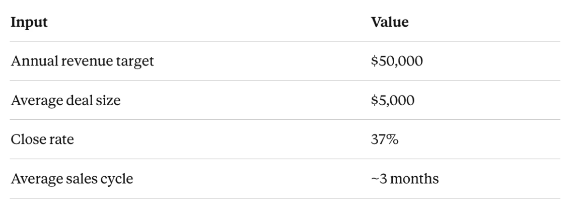
Working backwards:
- Deals needed to win: $50,000 / $5,000 = 10 deals per year
- Deals needed to start: 10 / 0.37 = ~27 deals per year
- Monthly lead flow required: 27 / 12 = ~2.3 new deals per month
And by Little’s Law, the steady-state pipeline you will carry at any point in time:
Pipeline size: 2.3 deals/month × 3 months = ~7 deals in flight
That is your operating baseline. If your pipeline consistently has fewer than 7 active deals, you will miss your number. If it has many more, something else is off: deals are stalling, your cycle time is longer than you think, or you are counting opportunities that are not real.
Keep in mind that “consistently” is doing real work in that sentence. A snapshot of your pipeline on any given day will vary. What you are looking for is a pattern over time, not a precise daily count.
Why This Matters More Than You Think
The reason this framework is so useful is not the arithmetic. It is the clarity it forces. There are only four variables in this system:
- Lead flow (how many new deals enter per period)
- Sales cycle (how long deals take)
- Close rate (what fraction win)
- Deal size (revenue per closed deal)
Every sales outcome you care about is a function of these four things. Nothing else. When your pipeline is unhealthy, it is because one or more of these is broken.
This means you can diagnose problems precisely, and more importantly, you can model what happens when you improve them. Rather than reacting to a bad quarter with a flurry of activity, you can ask a more useful question: which variable moved, and why?
Running the Levers
Here is where it gets interesting. Let’s take the baseline above and see what happens when you pull different levers.
Lever 1: Shorten the Sales Cycle
What if you cut your average sales cycle from 3 months to 2 months, by tightening your discovery process, getting to proposals faster, or reducing decision-making friction?
- Lead flow stays at 2.3/month
- Pipeline size drops: 2.3 × 2 = 4.6 deals (instead of 7)
- You are closing deals faster, so you reach your annual target with less capital tied up in pipeline
Shorter cycles do not just feel better. They make your whole business more capital-efficient. You need less pipeline to generate the same revenue.
Lever 2: Improve Close Rate
What if you improve close rate from 37% to 50%, through better qualification, stronger proposals, or more disciplined follow-up?
- Deals needed to start: 10 / 0.50 = 20 deals per year (instead of 27)
Monthly lead flow required: 20 / 12 = 1.7 new deals/month (instead of 2.3)
You need 26% fewer leads to hit the same number. For organizations where lead generation is the biggest bottleneck, this is significant. A better conversion process can substitute for a larger top-of-funnel.
Lever 3: Increase Lead Flow
What if you double your inbound or outbound efforts and bring in 4.5 new deals per month instead of 2.3?
- Deals won: 4.5 × 12 × 0.37 = 20 deals per year
Revenue: 20 × $5,000 = $100,000 (double your original target)
More leads, same close rate and cycle time, double the output. The math scales linearly, which is exactly what you want to verify before investing heavily in marketing or sales headcount.
The Variability Problem
Little’s Law works on averages, and averages can hide a lot. Two sales teams can have identical average cycle times and close rates and produce wildly different results, because one team’s numbers are stable and the other’s swing dramatically from period to period.
This is where control charts become useful. A control chart plots your key variables over time and shows not just the average but the expected range of normal variation. If your close rate runs between 30% and 45% month to month, that is probably just noise in the system. If it drops to 12% in a single quarter, that is a signal worth investigating.
The practical implication: when you use Little’s Law to set pipeline targets, treat the output as a center line, not a hard number. Build in a buffer that reflects how variable your inputs actually are. A team with stable, consistent metrics can run a leaner pipeline than one where results swing dramatically from period to period.
What Most Business Leaders Get Wrong
The most common mistake is treating pipeline size as the primary health metric. “We have $500K in pipeline” sounds good. But pipeline size without context is almost meaningless.
A $500K pipeline where deals average a 3-month cycle and a 40% close rate is very different from a $500K pipeline where deals drag on for 9 months at a 15% close rate. The math on those two scenarios points to entirely different businesses.
The right question is not “how big is our pipeline?” It is: “Given our close rate and cycle time, does our pipeline size imply the lead flow we need to hit our number?”
If the implied lead flow is lower than what you are actually generating, deals are stalling. If it is higher, you are probably losing opportunities before they are being tracked. Either way, you have a specific problem to solve, not a vague feeling.
A Practical Starting Point
If you have not done this math for your own business, here is where to start:
Step 1: Measure your four variables. Pull the last 6 to 12 months from your CRM. Calculate average deal size, close rate (won / total resolved), average cycle time (days from first contact to close or loss), and average new deals added per month. While you are at it, note how much each variable moves around from period to period. That spread matters just as much as the average.
Step 2: Apply Little’s Law. Multiply your average monthly deal flow by your average cycle time (in months). That is your expected steady-state pipeline count. Compare it to what you actually see. If they are very different, something in your measurement or process is off.
Step 3: Work backwards from your target. Take your revenue goal, divide by deal size to get deals needed, divide by close rate to get deals that need to enter the pipeline, divide by cycle time to get required monthly lead flow. Now you have a number you can actually manage to.
Step 4: Model the levers. Pick the one variable that seems most improvable. Rerun the math with a realistic improvement and see what it does to your required pipeline and activity levels. Then ask whether you have a mean problem (the average needs to move) or a variance problem (the average is fine but the swings are too wide). Those are different problems with different solutions.
The Bottom Line
Little’s Law gives you a model, not a crystal ball. The value is not a perfect prediction. It is a shared language for understanding why your pipeline looks the way it does, and a principled basis for deciding where to focus.
Most sales conversations are about tactics: which outreach sequence, which pricing page, which discount to offer. This framework pulls you up to the level of the system. And once you see it as a system, you stop reacting to individual deals and start engineering the whole thing.
That is the difference between leadership teams that are always surprised by their quarterly numbers and ones that are not.